Home
Introduction
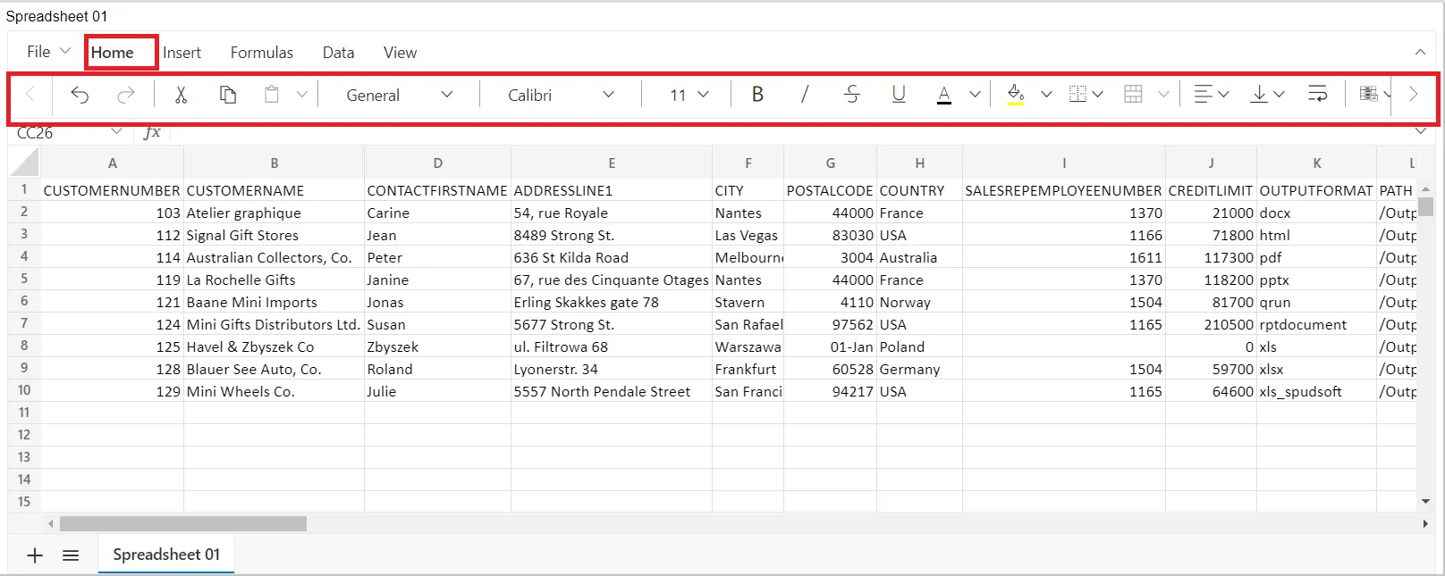
The Home menu is the second menu in the Excel menu bar. The Home ribbon items include options for formatting font, color, conditional formatting, number type, and more. All these functions help one in performing various effective calculations.
The home menu provides many features to users including changing the font type, size, and color, Setting text to be bold or underlined, Adding or removing highlighting color around text, and Justify text on the page to be left, center, or right-aligned, Add bullet point or numbered lists, Increase or decrease line and paragraph spacing, Increase or decrease text indentation, Add, change, or remove borders around text, text boxes, and tables, Add or modify heading types, Insert a horizontal line.
Prerequisite
Users will require the following dataset to understand edit spreadsheet scenarios:
Customers.cds dataset
Download Customers.zip file-click here
Permissions
For the spreadsheet widget, certain permissions need to be set. Before adding any general changes on the spreadsheet, ensure you set the following permissions on the widget:
- Uncheck “Allow Protection”
- Check “Show Ribbon”
- Check “Allow Editing”
To use the Home menu in the Spreadsheet follows the steps below:
Undo & Redo
Undo: The undo button in Spreadsheet reverts your worksheet to the state it was in just before you performed the most recent action. To use Undo for Windows, press Ctrl+Z.
Redo: Redo has the opposite effect, redoing what you’ve just undone, such as if you accidentally delete something. You can perform a redo using the Ctrl+Y.
Clipboard Group
Cut: In Excel, cutting data is defined as moving the data from one location to another, either to a different spot in the same worksheet, a separate worksheet in the same workbook, a different Excel workbook, or even a different application.
Copy: When you copy a cell, the selected cell data remains in its original location and is added to a temporary storage area called the Clipboard. You can use the Copy Sheet icon to copy entire worksheets (also known as sheets), to other locations in the same or a different workbook. If you want to copy something, then first you select the same thing, then by clicking on a copy it will be added to other places.
Paste: By default when you copy (or cut) and paste in Excel, everything in the source cell or range—data, formatting, formulas, validation, comments—is pasted to the destination cell(s). This is what happens when you press CTRL+V to paste. You have many other paste options, depending on what you copy.
Number Formatting
This option helps to choose how the values in a cell are displayed. Provides a list of all the available number formats. The built-in number formats are: General, Number, Currency, Accounting, Short Date, Long Date, Time, Percentage, Fraction, Scientific and Text.
General: The default number format that Excel applies when you type a number. For the most part, numbers that are formatted with the General format are displayed just the way you type them.
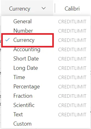
To show numbers as currency, you can apply either the Currency format or the Accounting format.
Select the cells that you want to format to demonstrate we are using currency Formant in CreditLimit and then, in the Number group on the Home tab, click the down arrow in the General.
Choose Currency, as shown in the figure below:
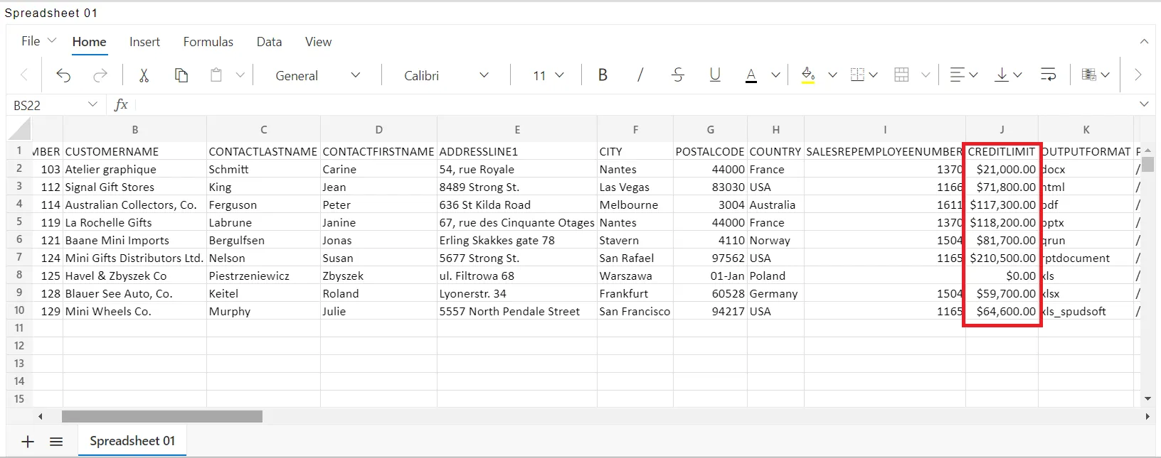
You can see that the decimal points appear aligned in the column. The currency symbol appears next to the first digit in the cell $ symbol is added in the CreditLimit column, as shown in the figure below:
Different types of formatting options with expressions are listed below:
| Types | Format |
|---|---|
| General(default) | NA |
| Number | 0.00 |
| Currency | $#,##0.00 |
| Accounting | _($* #,##0.00_);_($* (#,##0.00);_($* "-"??_);_(@_) |
| ShortDate | mm-dd-yyyy |
| LongDate | dddd, mmmm dd, yyyy |
| Time | h:mm:ss AM/PM |
| Percentage | 0.00% |
| Fraction | # ?/? |
| Scientific | 0.00E+00 |
| Text | @ |
Custom Number Formatting
Spreadsheet supports custom number formats to display your data as numbers, dates, times, percentages, and currency values. If the pre-defined number formats do not meet your needs, you can set your custom formats using the custom number formats dialog
Different types of Custom Number formatting with respected expressions are listed below:
| Types | Format |
|---|---|
| General(default) | NA |
| Number | 0 |
| Number | 0.00 |
| Number | #,##0 |
| Number | #,##0.00 |
| Number | #,##0_);(#,##0) |
| Number | #,##0_);[Red](#,##0) |
| Number | #,##0.00_);(#,##0.00) |
| Number | #,##0.00_);[Red](#,##0.00) |
| Currency | $#,##0_);($#,##0) |
| Currency | $#,##0_);[Red]($#,##0) |
| Currency | $#,##0.00_);($#,##0.00) |
| Currency | $#,##0.00_);($#,##0.00) |
| Percentage | 0% |
| Percentage | 0.00% |
| Scientific | 0.00E+00 |
| Scientific | ##0.0E+0 |
| Fraction | # ?/? |
| Fraction | # ??/?? |
| ShortDate | dd-mm-yy |
| Custom | dd-mmm-yy |
| Custom | dd-mmm |
| Custom | mmm-yy |
| Custom | h:mm AM/PM |
| Custom | h:mm:ss AM/PM |
| Custom | h:mm |
| Custom | h:mm:ss |
| Custom | dd-mm-yy h:mm |
| Custom | mm:ss |
| Custom | mm:ss.0 |
| Text | @ |
| Custom | [h]:mm:ss |
| Accounting | _($* #,##0_);_($* (#,##0);_($* "-"_);_(@_) |
| Accounting | _(* #,##0_);_(* (#,##0);_(* "-"_);_(@_) |
| Accounting | _($* #,##0.00_);_($* (#,##0.00);_($* "-"??_);_(@_) |
| Accounting | _(* #,##0.00_);_(* (#,##0.00);_(* "-"??_);_(@_) |
Font
Each type of font and style has a specific purpose. It directly reflects the tone of what we are trying to show in a spreadsheet. The Syncfusion JavaScript Spreadsheet supports several custom font style options like font family, font size, bold, italics, color, and underline.
The default font family is Calibri, and the default font size is 11 pt.
Font Size: In this font size option we can adjust text size according to us. Select the text that you want to adjust and go to the font size and size it accordingly.
Bold: (Ctrl+B) You can use this command to bold your selected text.
Italic: (Ctrl+I) You can use this command to italic your selected text.
Strikethrough: It refers to drawing a line through a value in a cell.
Underline (Ctrl+U) With the help of these options, your selected text will be underlined.
Text Color: Use this tool to change the text color. Clicking on the drop-down button, you get more colors.
Fill Colour: Fill color is useful to call attention to a specific cell or range of cells. You can use it to highlight the result of a calculated formula or a specific value. You can find the fill color option in the Home tab of the ribbon in the Spreadsheet control.
Borders
Button with Drop-Down. The button applies a border to the current selection. You can add borders around a cell or range of cells to define a section of a worksheet or a table. The different types of border options available in the spreadsheet are,
| Types | Action |
|---|---|
| Top Border | Specifies the top border of a cell or range of cells. |
| Left Border | Specifies the left border of a cell or range of cells. |
| Right Border | Specifies the right border of a cell or range of cells. |
| Bottom Border | Specifies the bottom border of a cell or range of cells. |
| No Border | Used to clear the border from a cell or range of cells. |
| All Border | Specifies all borders of a cell or range of cells. |
| Horizontal Border | Specifies the top and bottom border of a cell or range of cells. |
| Vertical Border | Specifies the left and right border of a cell or range of cells. |
| Outside Border | Specifies the outside border of a range of cells. |
| Inside Border | Specifies the inside border of a range of cells. |
You can also change the color, size, and style of the border.
You can also change the color, size, and style of the border. The size and style supported in the spreadsheet are,
| Types | Action |
|---|---|
| Thin | Specifies the 1px border size (default). |
| Medium | Specifies the 2px border size. |
| Thick | Specifies the 3px border size. |
| Solid | Used to create the solid border (default). |
| Dashed | Used to create the dashed border. |
| Dotted | Used to create the dotted border. |
| Double | Used to create the double border. |
Merge Cell: Merge cells allows users to span two or more cells in the same row or column into a single cell. When cells with multiple values are merged, top-left most cell data will be the data for the merged cell.
The available merge options in the spreadsheet are,
| Type | Action |
|---|---|
| Merge All | Combines all the cells in a range into a single cell (default). |
| Merge Horizontally | Combines cells in a range as row-wise. |
| Merge Vertically | Combines cells in a range as column-wise. |
| UnMerge | Splits the merged cells into multiple cells. |
Alignment
Horizontal Alignment: To enhance the visual presentation of your data, you can align text in a cell vertically or horizontally. To align text vertically pick the top, middle or bottom align, and to align text horizontally pick left, center or right align.
| Type | Action |
|---|---|
| Align Left | Align text to the left edge of the cell. |
| Center | Aligns text to the middle of the cell. |
| Align Right | Aligning text to the right edge of the cell. |
Vertical alignment: Vertical alignment is used to align the text vertically in a cell. The default vertical alignment is the bottom. We have tree alignment options:
| Type | Action |
|---|---|
| Top Align | Align text to the top of the cell. |
| Middle Align | Align text to the center of the cell. |
| Bottom Align | Align text to the bottom of the cell. |
Wrap Text: To make text appear on multiple lines in a cell, you can apply wrap text to the cell. So, that the text wraps automatically or you can enter a manual line break using the ALT + ENTER key in edit mode.
Conditional Formatting
Conditional formatting helps you to format a cell or range of cells based on the conditions applied. Conditional formatting has the following types in the spreadsheet:
Highlight cells rules: Highlight cells rules option in the conditional formatting enables you to highlight cells with a preset color depending on the cell’s value. The options can be given for the highlight cells rules as type, GreaterThan, LessThan, Between, EqualTo, ContainsText, DateOccur, Duplicate, Unique.
The preset colors can be used for formatting styles:
- RedFT: Light Red Fill with Dark Red Text
- YellowFT: Yellow Fill with Dark Yellow Text
- GreenFT: Green Fill with Dark Green Text
- RedF: Red Fill
- RedT: Red Text.
Top-bottom rules: Top-bottom rules option in the conditional formatting allows you to apply formatting to the cells that satisfy a statistical condition with other cells in the range.
This options can be given for the top bottom rules as type: Top10Items, Bottom10Items, Top10Percentage, Bottom10Percentage, BelowAverage, AboveAverage.
Data Bars: You can apply data bars to represent the data graphically inside a cell. The longest bar represents the highest value and the shorter bars represent the smaller values.
This options can be given for the data bars as type, BlueDataBar, GreenDataBar, OrangeDataBar, LightBlueDataBar, PurpleDataBar.
Color Scales: Using color scales, you can format your cells with two or three colors, where different color shades represent the different cell values. In the Green-Yellow-Red(GYR) Color Scale, the cell that holds the minimum value is colored as red. The cell that holds the median is colored yellow, and the cell that holds the maximum value is colored green. All other cells are colored proportionally.
This options can be given for the color scales as type, GYRColorScale, RYGColorScale, GWRColorScale, RWGColorScale, BWRColorScale, RWBColorScale, WRColorScale, RWColorScale, GWColorScale, WGColorScale, GYColorScale, YGColorScale.
Icon Sets: Icon sets will help you to visually represent your data with icons. Every icon represents a range of values. In the Three Arrows(colored) icon, the green arrow icon represents the values greater than 67%, the yellow arrow icon represents the values between 33% to 67%, and the red arrow icon represents the values less than 33%.
This options can be given for the icon sets as type, ThreeArrows, ThreeArrowsGray, FourArrowsGray, FourArrows, FiveArrowsGray, FiveArrows, ThreeTrafficLights1, ThreeTrafficLights2, ThreeSigns, FourTrafficLights, FourRedToBlack, ThreeSymbols, ThreeSymbols2, ThreeFlags, FourRating, FiveQuarters, FiveRating, ThreeTriangles, ThreeStars, FiveBoxes.
Clear Rules: You can clear the defined rules by using one of the following ways, Using the Clear Rules option in the Conditional Formatting button of the HOME Tab in the ribbon to clear the rule from selected cells.
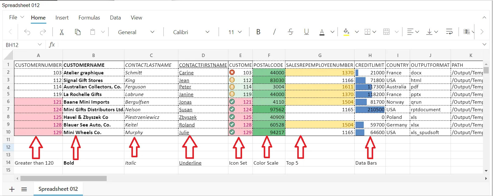
The output of the Home menu function, as shown in the figure below:
Clear: Clear feature helps you to clear the cell contents (formulas and data), and formats (including number formats, conditional formats, and borders) in a spreadsheet. When you apply clear all, both the contents and the formats will be cleared simultaneously.
You can apply the clear feature by Selecting the clear icon in the Ribbon toolbar under the Home Tab.
Clear has the following types in the spreadsheet,
| Options | Uses |
|---|---|
| Clear All | Used to clear all contents, formats, and hyperlinks. |
| Clear Formats | Used to clear the formats (including number formats, conditional formats, and borders) in a cell. |
| Clear Contents | Used to clear the contents (formulas and data) in a cell. |
| Clear Hyperlinks | Used to clear the hyperlink in a cell. |
Sorting
Sorting helps arrange the data to a specific order in a selected range of cells. In the active Spreadsheet, select a range of cells to sort by cell value. The range sort can be done in any of the following ways:
Select the sort item in the Ribbon toolbar and choose the ascending or descending item.
Right-click the sheet, select the sort item in the context menu, and choose the ascending/descending item.
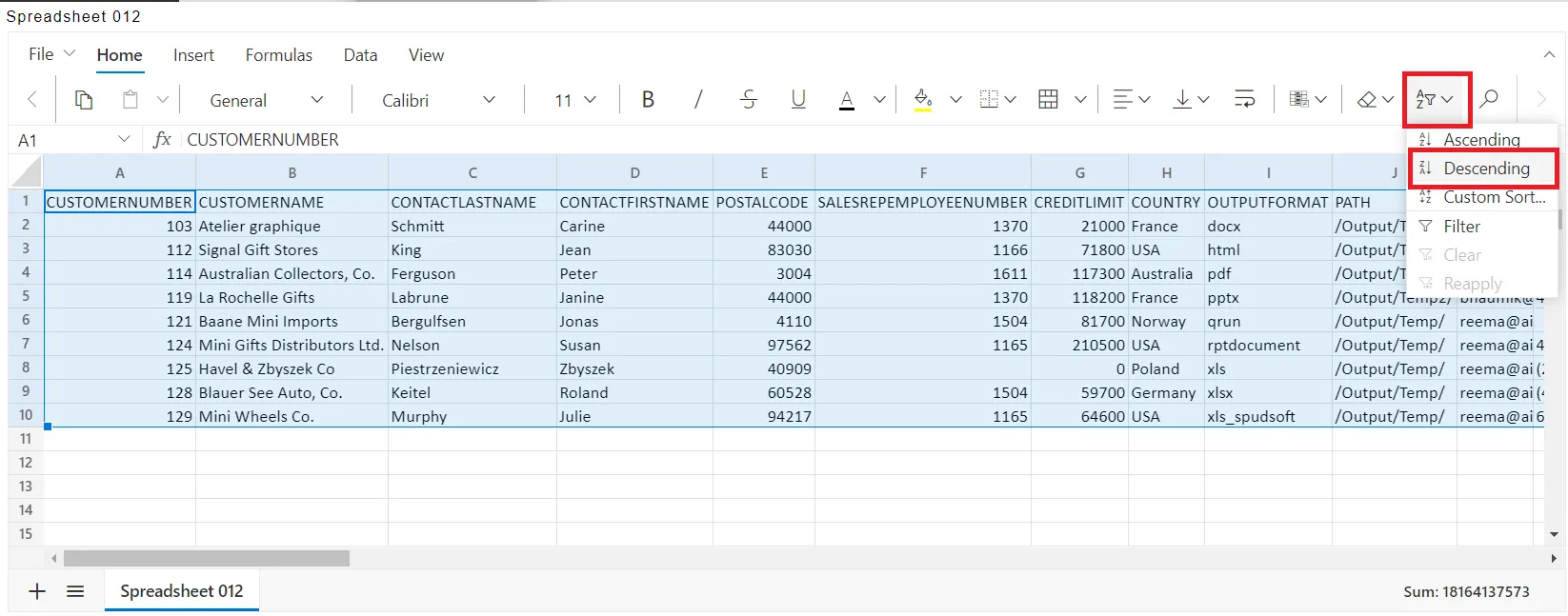
The cell values can be sorted in Ascending or Descending orders. For demonstration, we are using Descending Order Sorting in the Customer Spreadsheet.
Select all the data of the spreadsheet go to Sort & Filter option and in the dropdown select the descending Order, as shown in the figure below:
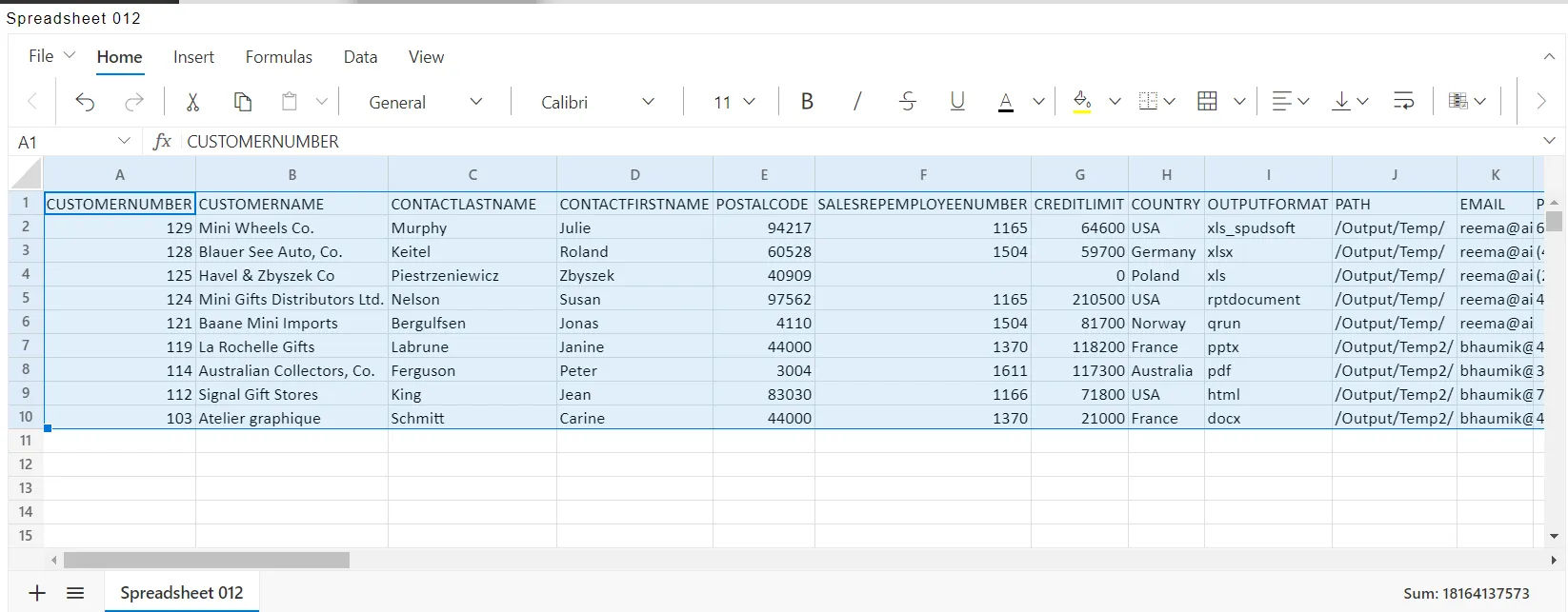
The output of the sorting is shown in the figure below:
Custom sort: The custom sort dialog helps sort multiple columns in the selected range by utilizing the rich UI. This dialog will have appeared while choosing the Custom sort… from the Ribbon item or context menu item. By default, sort criteria with the first column name from the selected range will have appeared in the dialog on initial load and it cannot be removed.
You can add multiple criteria using the Add Column button at the bottom of the dialog. Thus, multiple columns can be specified with different sort orders. The newly added sort criteria items can be removed using the delete icons at the end of each item.
Filtering
Filtering helps you to view specific rows in the spreadsheet by hiding the other rows. In the active Spreadsheet, select a range of cells to filter by the value of the cell.
The filtering can be done in any of the following ways:
Select the filter item in the Ribbon toolbar.
Right-click the sheet, and select the filter item in the context menu.
Use Ctrl + Shift + L keyboard shortcut to apply the filter.
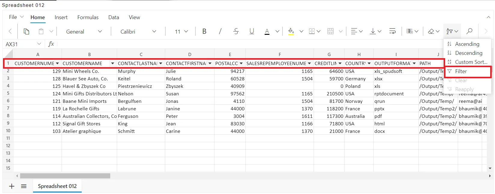
Select all the data of the spreadsheet go to Sort & Filter option and in the dropdown select the filter option, the output is shown in the figure below:
Filter by cell value: To apply a filter for a cell value, right-click the cell and choose the filter -> Filter By Selected Cell’s Value option from the menu. It applies the filter based on the value of the selected cell in the current sheet.
Clear filter: After applying the filter to a certain column, you may want to clear it to make all filtered rows visible again. It can be done by Choose Clear option in the ribbon toolbar under Filter and Sort. It clears the filters applied in the spreadsheet for all fields.
Reapply filter: When you want to reapply the filter after some changes happened in the rows. It can be done in the following ways:
You can choose Reapply option in the ribbon toolbar under Filter and Sort to reapply the filtered columns again.
You can right-click on a filtered cell and choose Reapply option from the context menu. It reapplies the filters again in the Spreadsheet for all the fields.