Insert

Introduction

Insert Tab helps you to insert an image, Chart, and Hyperlink in the spreadsheet.

Prerequisite

Users will require to follow the dataset to understand edit spreadsheet scenarios.

Customers.cds dataset

Download Customers.zip file

Permissions

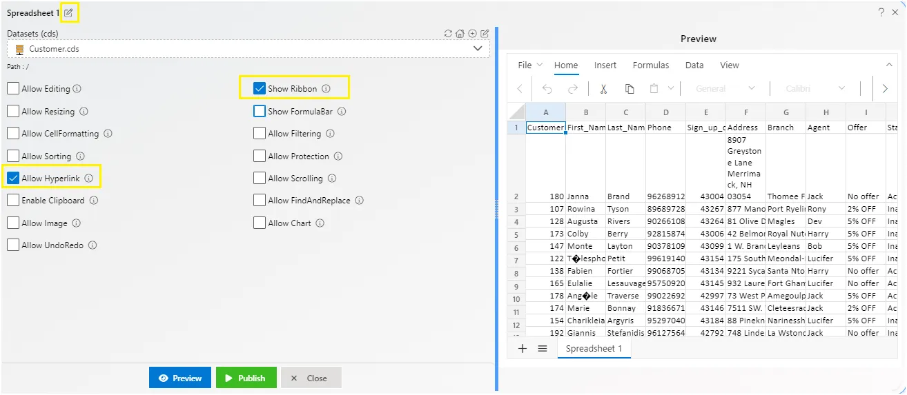
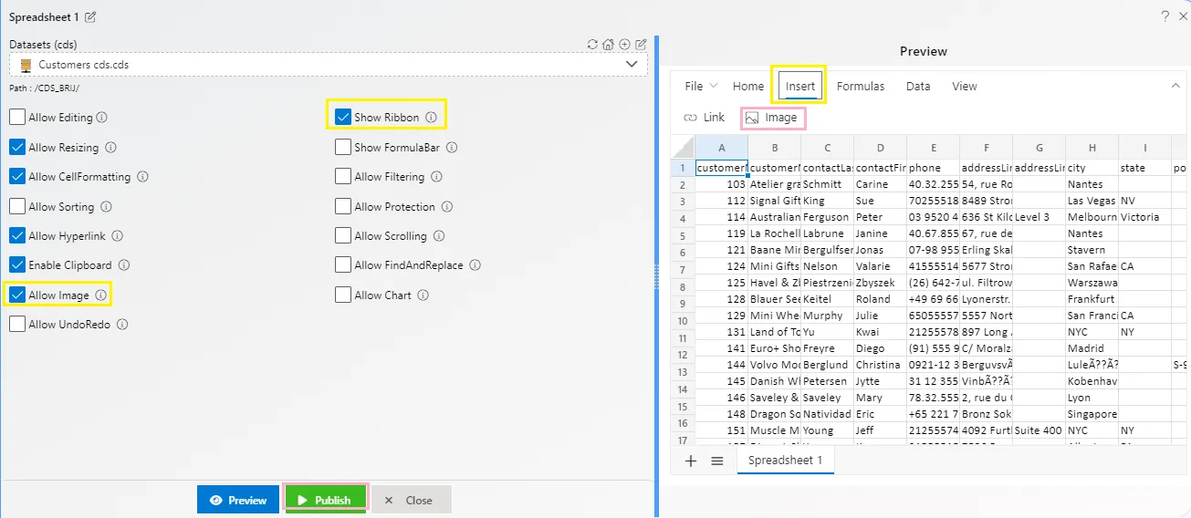
For the spreadsheet widget, certain permissions need to be set. Before adding any link, image, chart on the spreadsheet, ensure you set the following permissions on the widget:

• Uncheck “Allow Protection”
• Check “Show Ribbon”
• Check “Allow Editing”
• Check “Allow Hyperlink”
• Check “Allow Image”
• Check “Allow Chart”

Insert Tab has three Functionalities:

1. Hyperlink
2. Image
3. Chart

The following points contain steps to add the Hypelink, Image and Chart in the Spreadsheet.

1. Hyperlink

A hyperlink is used to navigate to web links or cell references within the sheet or to other sheets in the Spreadsheet. To quickly access related information in another file or on a web page, you can insert a hyperlink in a worksheet cell.

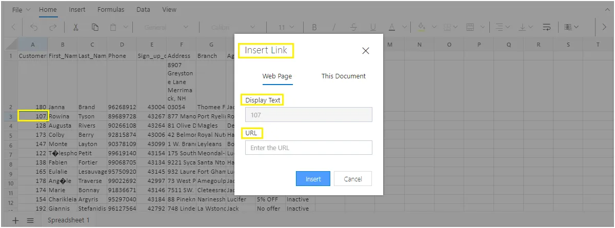
Insert Link: You can insert a hyperlink in a worksheet cell for quick access to related information. In the active spreadsheet, click the cell where you want to create a hyperlink. Inserting a hyperlink can be done in any of the following ways:

• Select the INSERT tab in the Ribbon toolbar and choose the Link item.
• Right-click the cell and then click the Hyperlink item in the context menu, or you can press Ctrl+K. You can insert Hyperlinks using the Web Page and This Document.

A dialog box will pop up, as shown in the figure below:

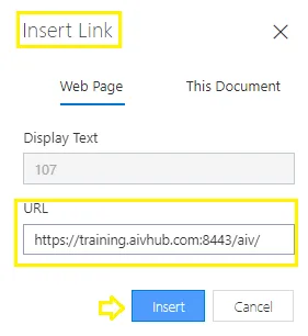
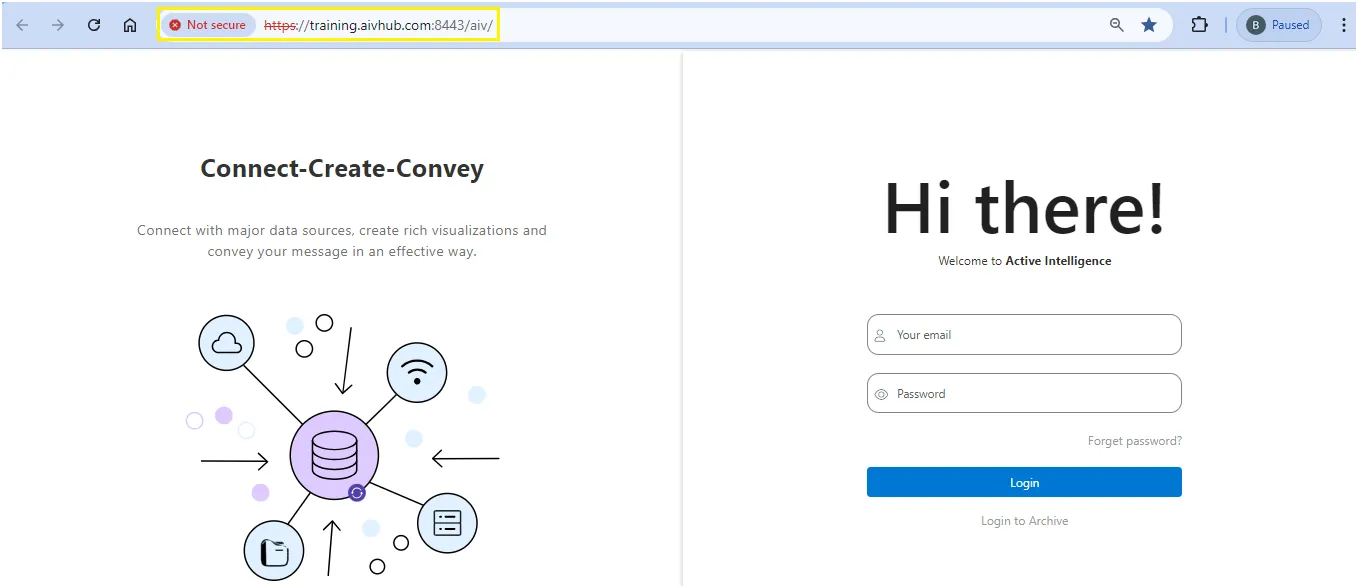
In the URL, copy the link where you want to redirect. Here we are using the link https://training.aivhub.com:8443/aiv/, as shown in the figure below:

Click on the Insert button, and the Hyperlink is added. You can see it in the figure below:

It will redirect you to the AIV login page, as shown in the figure below:

Insert Link using This Document

We are using the Customer Number Column in that select 103 CustomerNumber.Go to the Insert >> Link >> This Document.

In Cell Reference select the cell from which you want to redirect here we are selecting H2 Country Column and you can also select the sheet as per your requirement, as shown in the figure below:

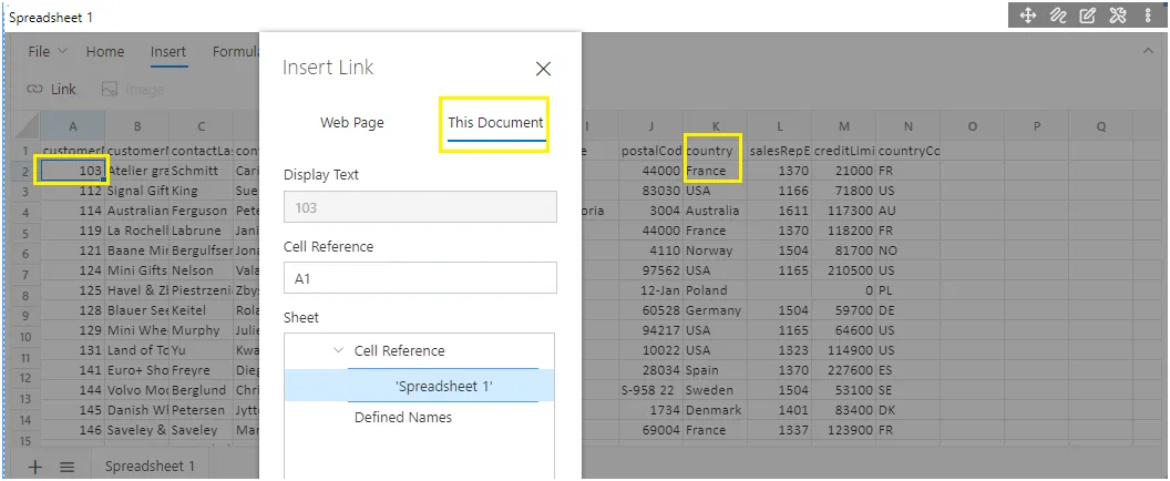
Click on Insert Button.

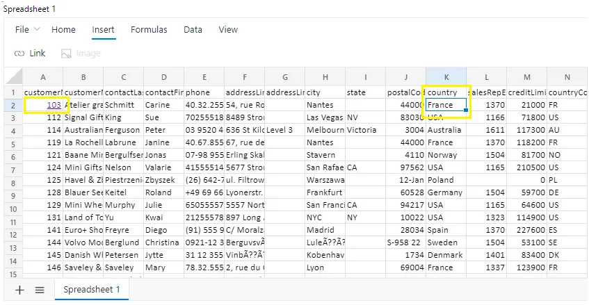
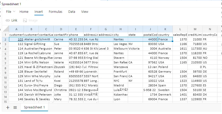
When you click on Customer Number 103, it will redirect you to the corresponding path in the “Path” column row, as illustrated in the figure below.:

Edit Hyperlink: You can change an existing hyperlink in your workbook by changing its destination or the text that is used to represent it.

In the active spreadsheet, Select the cell that contains the hyperlink that you want to change. Editing the hyperlink while opening the dialog can be done in any one of the following ways:

Select the INSERT tab in the Ribbon toolbar and choose the Link item.

Right-click on the Custome Number Column 103 cell and then click the Edit Hyperlink item in the context menu, or you can press Ctrl+K, as shown in the figure below:

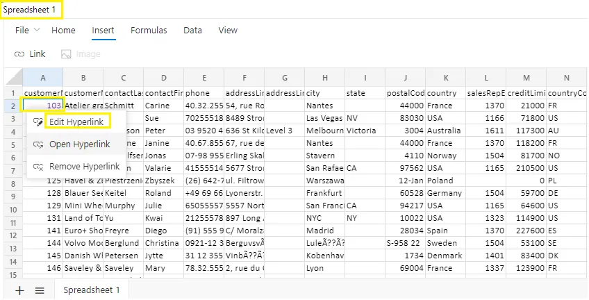
When you click on Edit Hyperlink it will display the pop-up, as shown in the figure below:

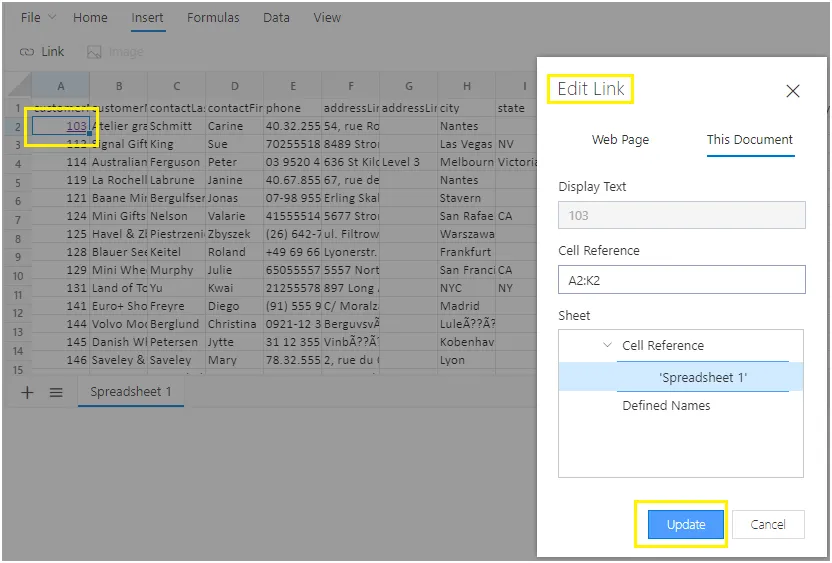
In the Edit Link dialog box, make the changes that you want, and click UPDATE., when you click on 103 it will now Select Row A2 to K2, as shown in the figure below:

Remove Hyperlink: Performing this operation removes a single hyperlink without losing the display text.

In the active spreadsheet, click the cell where you want to remove a hyperlink. remove hyperlinks can be done in any of the following ways:

Right-click the cell and then click the Remove Hyperlink item in the context menu.

On a worksheet, click the cell where you want to create a link. For demonstration, we are adding a hyperlink in the CustomerNumber column in the spreadsheet.

On the Insert tab, in the Links group, click the Link option. You can also right-click the cell and then click Hyperlink on the shortcut menu, or you can press Ctrl+K.

2. Image

You can insert a picture by selecting the “Pictures” button under the Illustrations group of the INSERT Tab in the ribbon. Adding images to a spreadsheet can enhance the visual appeal and help to convey information more clearly.

Insert Image: Image feature allows you to view and insert an image in a spreadsheet, and you can change the height and width of the image by resizing and moving it to another position. You can change the position of the image by drag and drop.

You can insert the image by selecting the Insert tab in the Ribbon toolbar and then choosing the Image tab. For demonstration we are adding an image of sales in the spreadsheet, as shown in the figure below:

Delete Image: If you want to delete the image, just select the image, and then press the Delete key.

3. Chart

A chart is a graphical representation of data, that organizes and represents a set of numerical or qualitative data. It mostly displays the selected range of data in terms of the x-axis and y-axis.

The chart feature allows you to view and insert a chart in a spreadsheet, and you can change the height and width of the chart by resizing and moving it to another position. You can change the position of the chart by drag and drop.

The types of charts available in the Spreadsheet are Column Chart, Bar Chart, Area Chart, Line Chart, Pie Chart, Scatter Chart .

Insert Chart: You can insert the chart by selecting the chart icon in the Ribbon toolbar under the Insert Tab.

Delete Chart: If you want to delete the chart, just select the chart, and then press the Delete key.

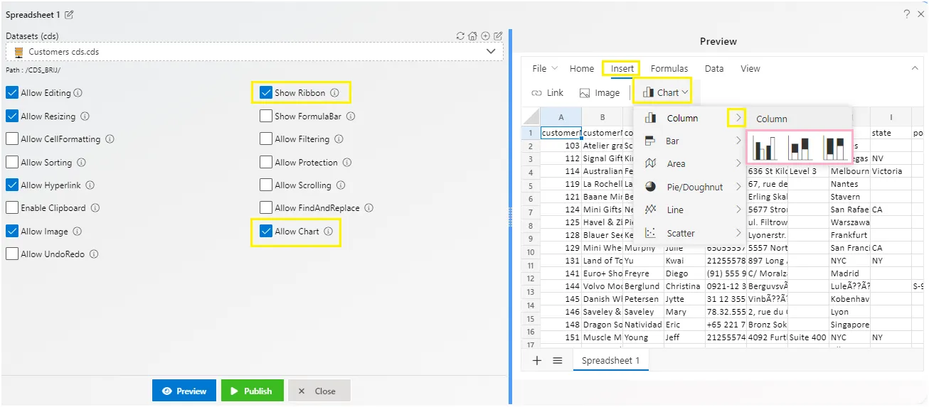
For demostration we are using ContactLastName and CreditLimit columns, select this both column than click on the Insert Tab >> Chart.

In the chart drop-down select the Column >> Clustered Column chart, as shown in the figure below:

The output of the Cluster Column chart, as shown in the figure below:

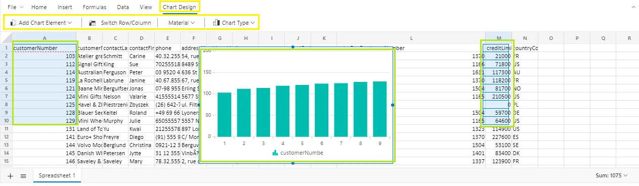
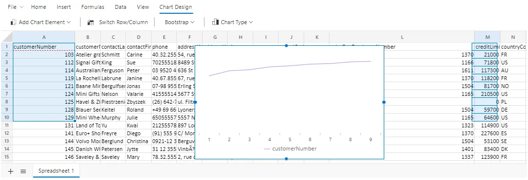
When you add a chart in the Spreadsheet Chart Design Tab and its property will be displayed, as shown in the figure below:

Add Chart Element: Using Add Chart Element we can Hide or show Axis, Axis Title, Chart Title, Data Labels, Gridlines, and Legends in the Chart which we have created.

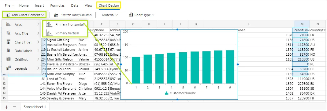
For example, we are hiding the category & value Axis of the chart which we have created.

Select your existing chart in a spreadsheet and go to Chart Design tab >> Add Chart Element dropdown >> Axis >> select Primary Horizontal and Primary Vertical, as shown in the figure below:

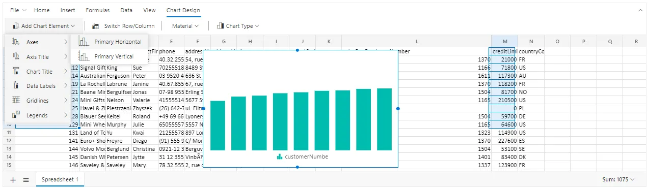
In the output you can see the category Axis and Value Axis will be hidden, as shown in the figure below:

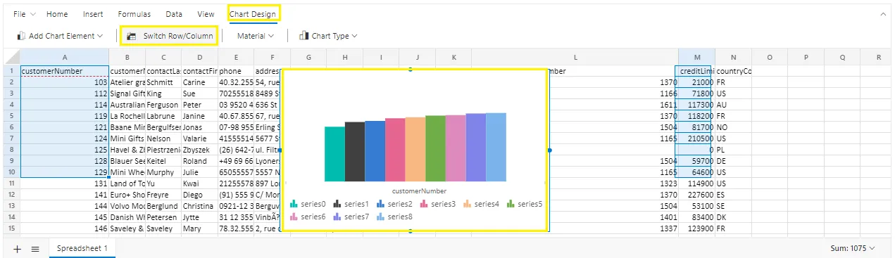
Switch Row/Column:

Material: Material is used for the theme you can apply different types of themes in the chart as per your requirement.

Select your existing chart in a spreadsheet and go to Chart Design tab >> Material >> Bootstrap, as shown in the figure below:

The output of the Bootstrap theme, as shown in the figure below:

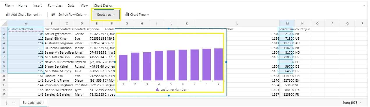
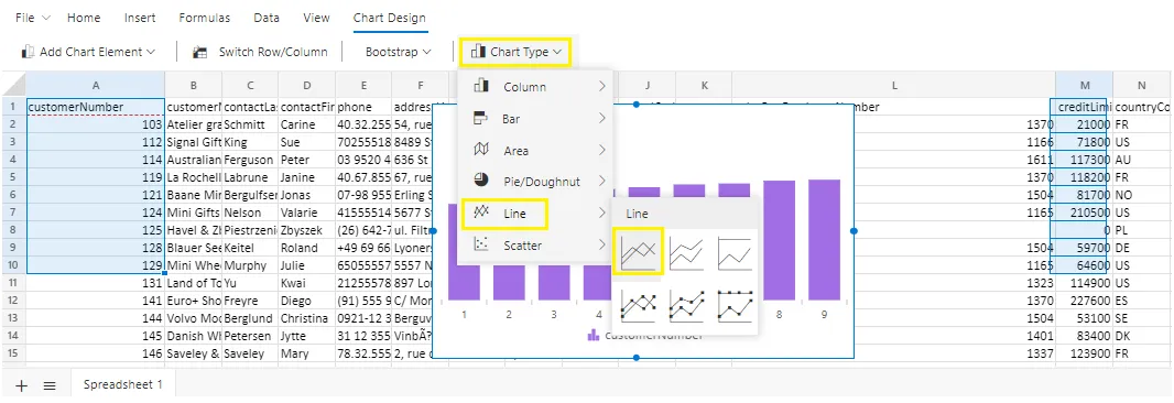
Chart Type: In Chart type you can change the chart type, as per your requirements.

Select your existing chart in a spreadsheet and go to Chart Design tab >> Chart Type >> Line Chart, as shown in the figure below:

The output of the Line Chart, as shown in the figure below: