View

Introduction

On the View menu, you customize the way spreadsheets appear on your screen. Options include displaying grid lines between cells, Hide Headers, Freeze Panes, Freeze Rows, and Freeze Columns.

Prerequisite

Users will require the following dataset to understand edit spreadsheet scenarios:

Sales.cds dataset

Download Sales.zip file

Upload this dataset in the Master Data >> Dataset section

Permissions

For the spreadsheet widget, certain permissions need to be set. Before adding any link, image, chart on the spreadsheet, ensure you set the following permissions on the widget:

Uncheck “Allow Protection”
Check “Show Ribbon”
Check “Allow Editing”

View Tab has Five Functionalities

Hide Headers
Hide Gridlines
Freeze Panes
Freeze Rows
Freeze Columns

1. Hide Headers

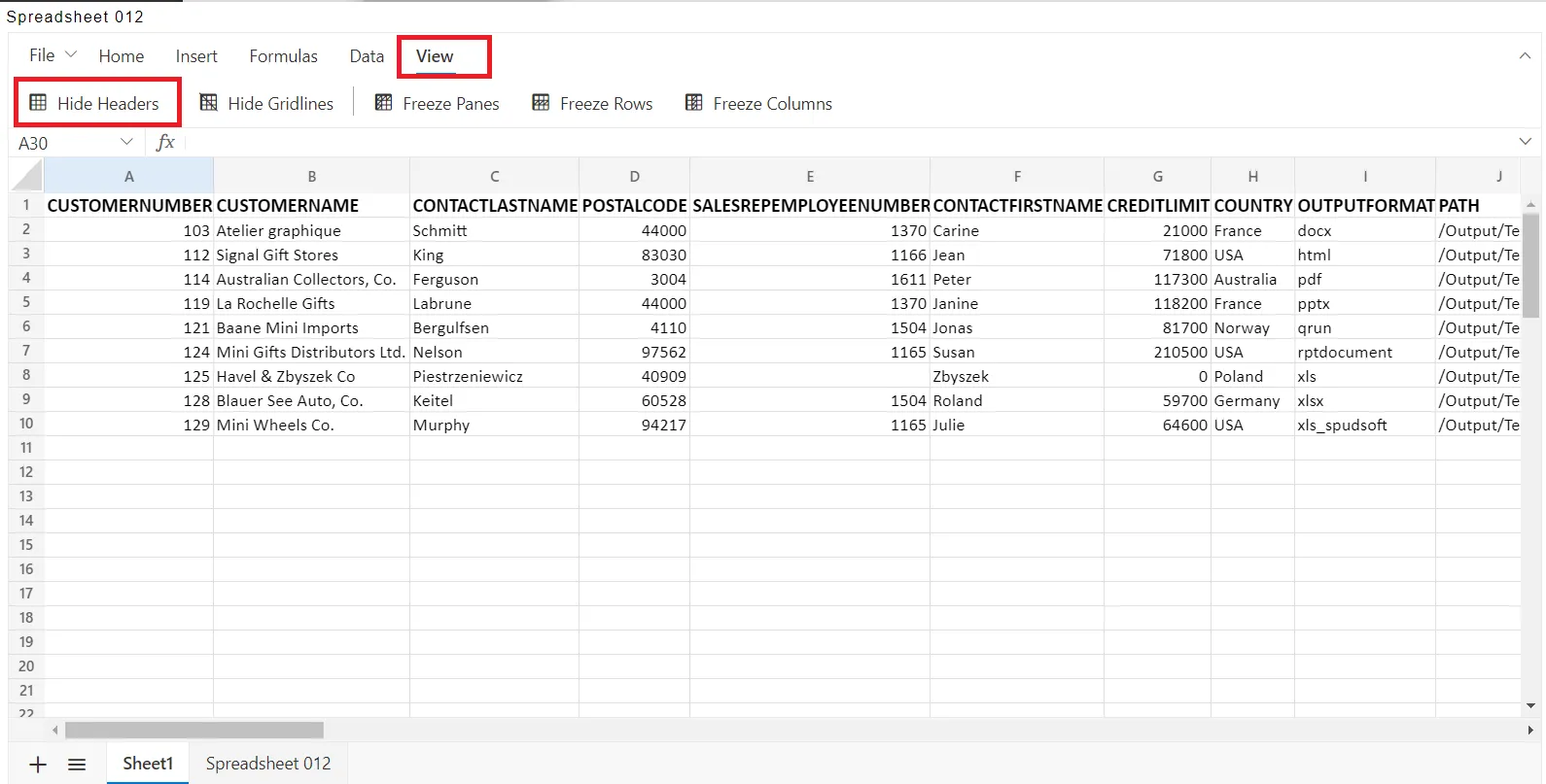
A header is information that appears at the top of each printed page. Hide Headers is used to Hide the Headers in the Spreadsheet. You can hide the Header of any worksheet to remove it from view. you can easily unhide hidden worksheets as needed.

Open the existing Spreadsheet which you already created.

For demonstration, we are using a customer spreadsheet that I already have created. Go to the View menu and select the Hide Header feature, as shown in the figure below:

When we click on the Hide Headers the output, as shown in the figure below:

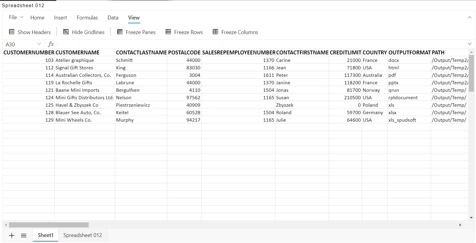
If you want to display the header click on the Show Headers property and you can see the Headers.

2. Hide Gridlines

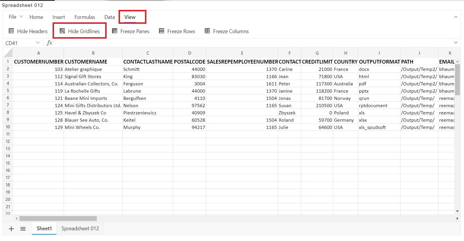
A spreadsheet contains cells and gridlines or grid bars represent the borders of these cells. It makes your spreadsheet clean and presentable. Although grid lines in excel have their benefits in some cases, it is better to hide them.

Open the existing Spreadsheet which you already created.

For demonstration, we are using a customer spreadsheet that I already have created. Go to the View menu and select the Hide Gridlines feature, as shown in the figure below:

when you click on the Hide Gridlines property it will hide all the Gridlines in the Spreadsheet, as shown in the figure below:

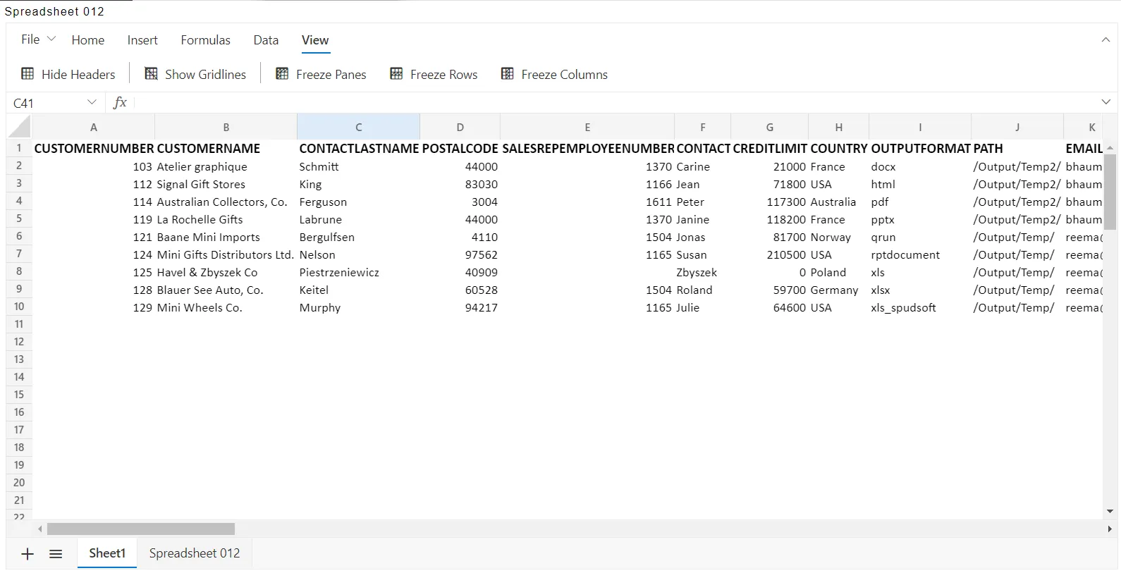
If you want to display the Gridlines click on the Show Gridlines property and you can see the Greenlines added to the spreadsheet.

3. Freeze Panes

Freeze Panes help you to keep particular rows or columns visible when scrolling the sheet content in the spreadsheet. In the active spreadsheet, click the cell where you want to create freeze panes. Freeze panes can be done by Selecting the View tab in the Ribbon toolbar and choosing the Freeze Panes item.

Open the existing Spreadsheet which you already created.

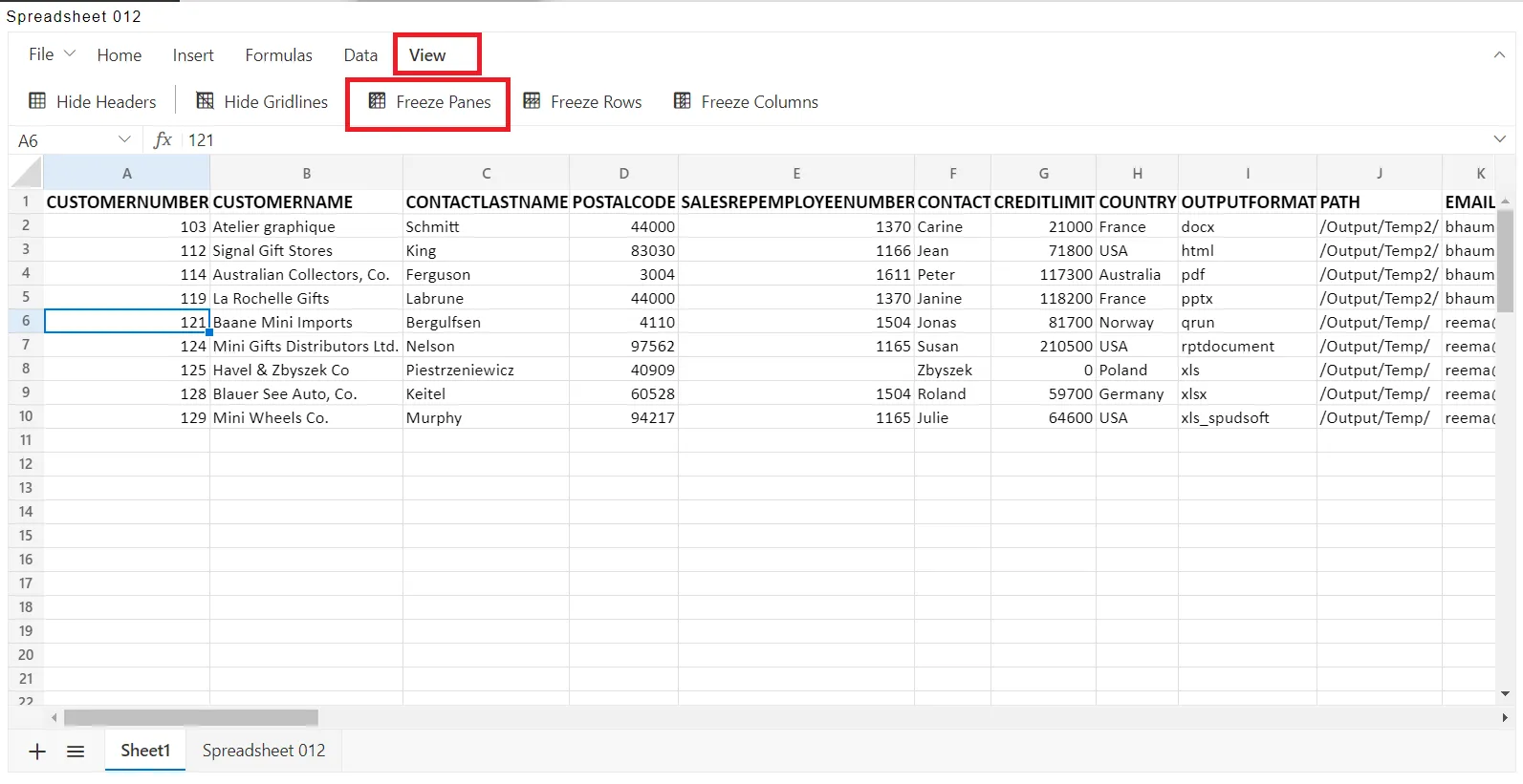
For demonstration, we are using a customer spreadsheet that I already have created. Click the cell where you want to freeze panes. Go to the View menu and select the Freeze Panes feature, as shown in the figure below:

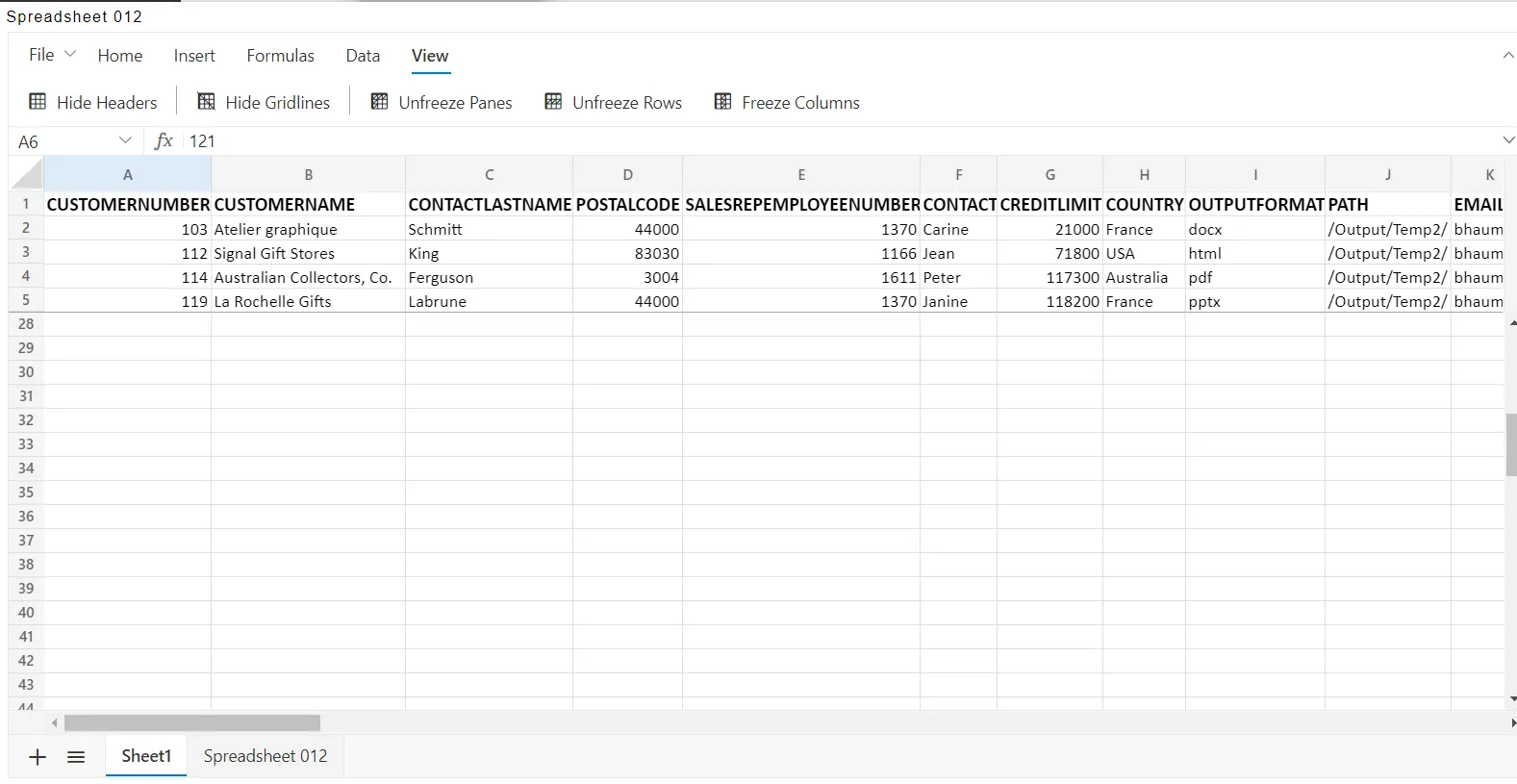
when you click on Freeze Panes it will freeze the certain number of rows & columns visible while scrolling the output of Freeze Panes, as shown in the figure below:

You can Unfreeze Panes by clicking on the Unfreeze property in the spreadsheet.

4. Freeze Rows

It allows you to keep a certain number of rows visible while scrolling vertically through the rest of the worksheet. In the active spreadsheet, select the cell where you want to create frozen rows. Frozen rows can be used by Selecting the View tab in the Ribbon toolbar and choosing the Freeze Rows item.

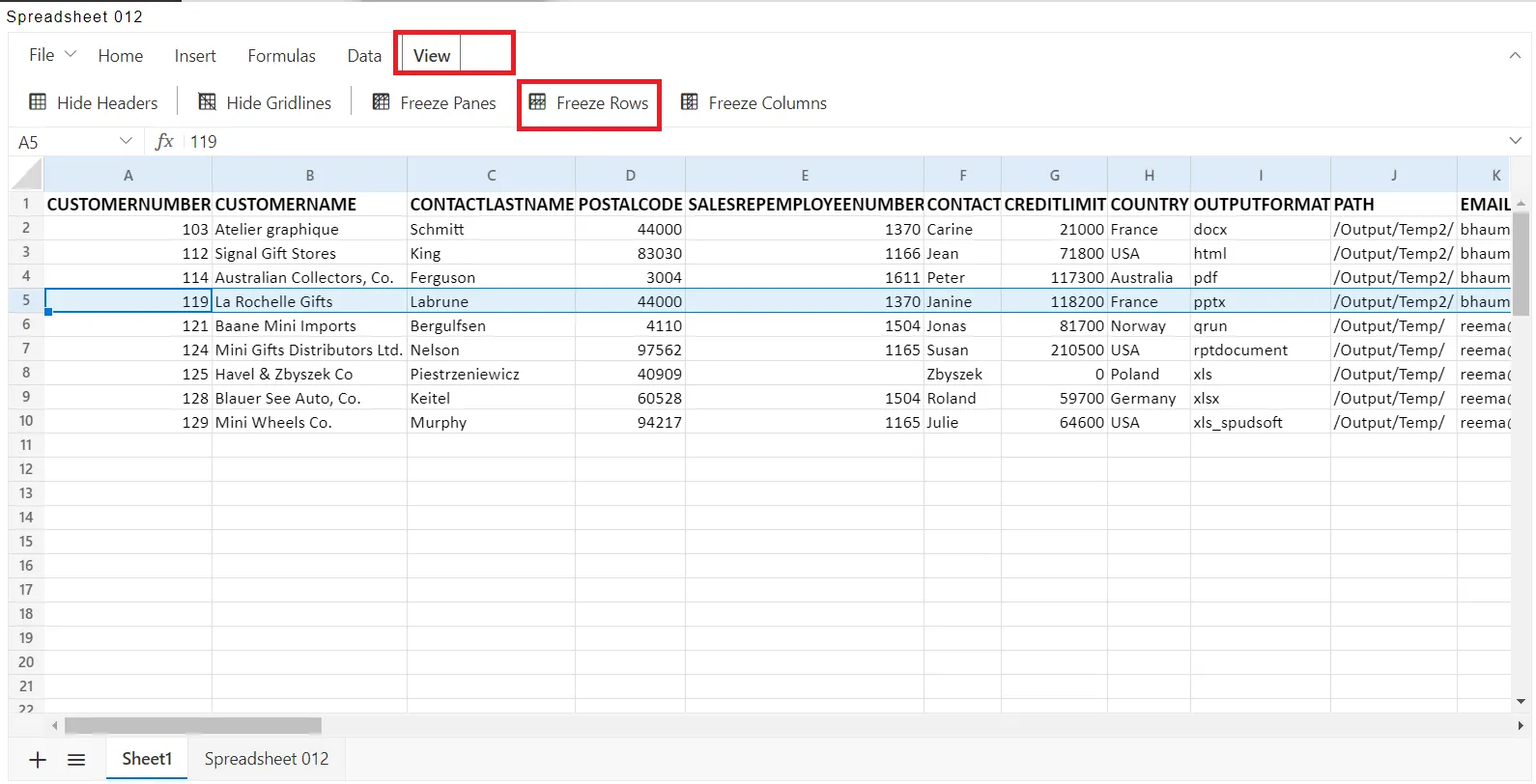
For demonstration, we are using a customer spreadsheet that I already have created. select the Rows where you want to Freeze Rows. Go to the View menu and select the Freeze Rows feature, as shown in the figure below:

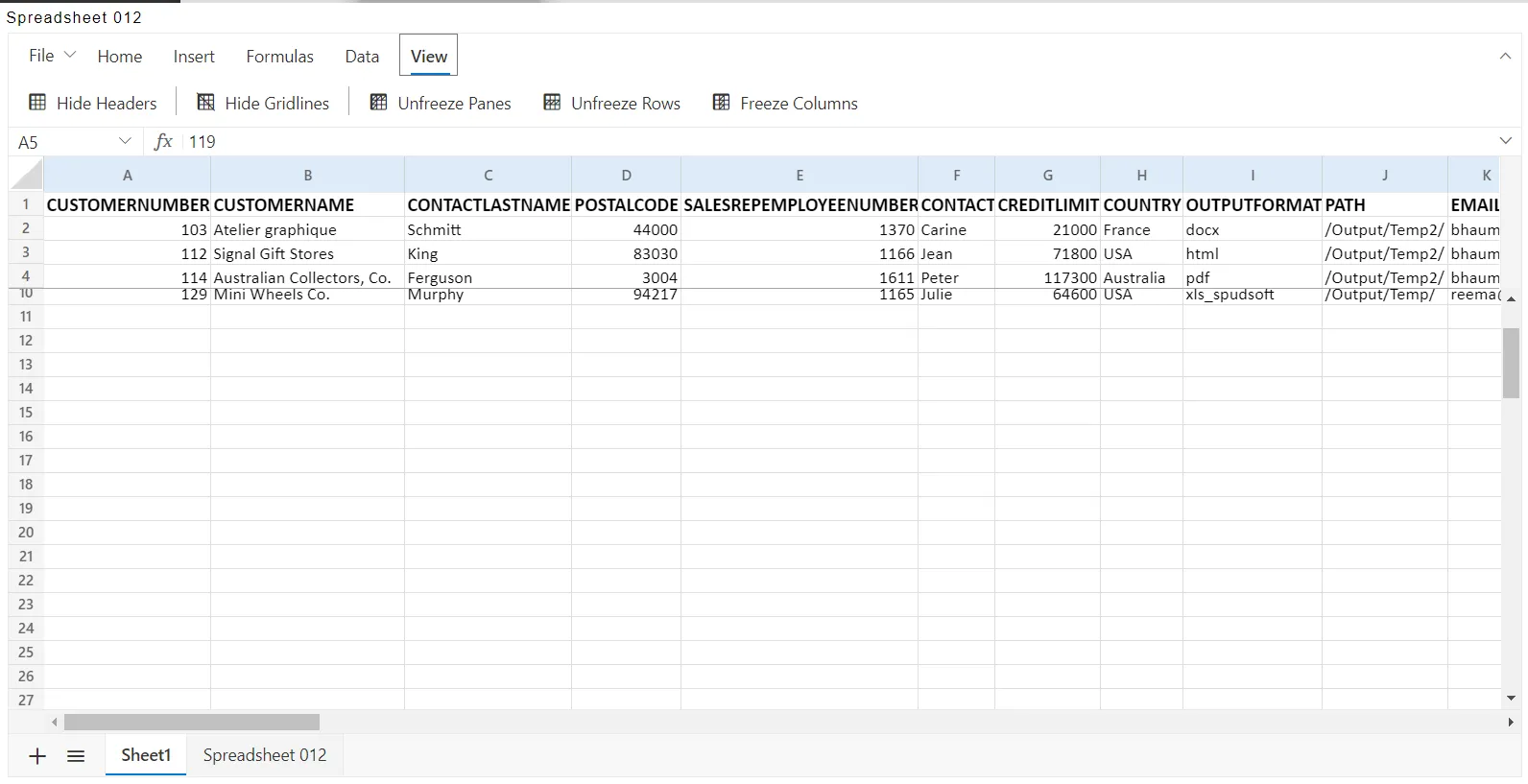
when you click on Freeze Rows it will freeze the certain number of rows & columns visible while scrolling the output of Freeze Panes, as shown in the figure below:

You can Unfreeze Rows by clicking on the Unfreeze Row property in the spreadsheet.

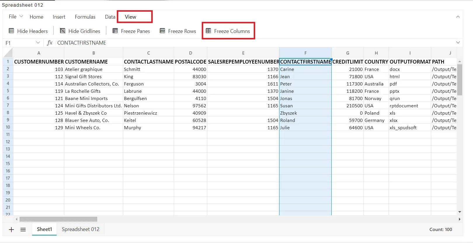
5. Freeze Columns

It allows you to keep a certain number of columns visible while scrolling horizontally through the rest of the worksheet.

In the active spreadsheet, select the cell where you want to create frozen columns. Frozen columns can be done by Selecting the View tab in the Ribbon toolbar and choosing the Freeze Columns item.

For demonstration, we are using a customer spreadsheet that I already have created. select the Column where you want to Freeze Column. Go to the View menu and select the Freeze Column feature, as shown in the figure below:

when you click on Freeze Column it will freeze the certain number of rows & columns visible while scrolling the output of Freeze Panes, as shown in the figure below:

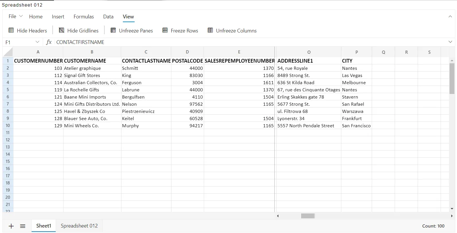
You can Unfreeze Column by clicking on the Unfreeze Column property in the spreadsheet.